Deterministic Policy Gradient Algorithms

Mathematical process about Deterministic Policy Gradient Algorithms.

目录

1. Policy Gradient
2. Stochastic Actor-Critic
3. Gradients of Deterministic Policies
4. Limit of the Stochastic Policy Gradient
5. Compatible Function Approximation
6. DDPG

An example of DDPG on pendulum

定义

符号

$r_{t}^{\gamma}=\displaystyle \sum_{k=t}^{\infty}\gamma^{k-t}r(s_{k},\ a_{k})$,其中$0<\gamma<1$
$V^{\pi}(s)=\mathrm{E}\left[r_{1}^{\gamma}|S_{1}=s;\pi\right]$
$Q^{\pi}(s,\ a)= \mathrm{E}\left[r_{1}^{\gamma}|S_{1}=s,\ A_{1}=a;\pi\right]$

常规条件

常规条件A.1: $p(s’|s,\ a)$ , $\nabla_{a}p(s’|s,\ a)$ , $\mu_{\theta}(s)$ , $\nabla_{\theta}\mu_{\theta}(s)$ , $r(s,\ a)$ , $\nabla_{a}r(s,\ a)$ , $p_{1}(s)$ 对任意变量 $s, a, s’$连续。

常规条件A.2: 存在 $b$ 和 $L$ 使得 $\displaystyle \sup_{s}p_{1}(s)<b,\ \displaystyle \sup_{a,s,s},\ p(s’|s,\ a)<b,\ \displaystyle \sup_{a,s}r(s,\ a)<b,\ \displaystyle \sup_{a,s,s},\ ||\nabla_{a}p(s’|s,\ a)||<L$, 并且 $\displaystyle \sup_{a,s}||\nabla_{a}r(s,\ a)||<L$。

模型性能

$$J(\pi_\theta)=\int_{\mathcal{S}}\rho^\pi(s)\int_{\mathcal{A}}\pi_\theta(s,\ a)r(s,\ a)dads=\mathbb{E}_{s\sim\rho^\pi,a\sim\pi_\theta}\left[r(s,\ a)\right]$$

其中$\rho^{\pi}(s’) := \int_{\mathcal{S}}\sum_{t=1}^{\infty}\gamma^{t-1}p_{1}(s)p(s\rightarrow s’,\ t,\ \pi)\mathrm{d}s$，成为折扣状态分布。论文中假设$\mathcal{A}=\mathbb{R}^m$，$\mathcal{S}$为$\mathbb{R}^b$的一个紧子集。有界闭集就是紧集。

1. Policy Gradient

$$\nabla_{\theta}J(\pi_{\theta})=\int_{\mathcal{S}}\rho^{\pi}(s)\int_{\mathcal{A}}\nabla_{\theta}\pi_{\theta}(s,\ a)Q^{\pi}(s,\ a)d{\it a}d{\it s}=\mathrm{E}_{s\sim\rho^{\pi},a\sim\pi_{\theta}}\left[\nabla_{\theta}\log\pi_{\theta}(s,\ a)Q^{\pi}(s,\ a)\right]$$

$\it Proof.$ 首先，

$$V^{\pi}(s)=\int_{\mathcal{A}}\pi_\theta(s,\ a)Q^\pi(s,\ a)da$$

对$\theta$求导，

$$\begin{split} &\nabla_{\theta}V^{\pi}(s)\\ &=\int_{\mathcal{A}}\left[\nabla_{\theta}\pi_\theta(s,\ a)Q^\pi(s,\ a)+\pi_\theta(s,\ a)\nabla_{\theta}Q^\pi(s,\ a)\right]da\\ &=\int_{\mathcal{A}}\left[\nabla_{\theta}\pi_\theta(s,\ a)Q^\pi(s,\ a)+\pi_\theta(s,\ a)\nabla_{\theta}\left[r(s,\ a)+\int_{\mathcal{S}}\gamma p(s\rightarrow s',\ 1,\ a)V^{\pi}(s')ds'\right]\right]da\\ &=\int_{\mathcal{A}}\left[\nabla_{\theta}\pi_\theta(s,\ a)Q^\pi(s,\ a)+\pi_\theta(s,\ a)\int_{\mathcal{S}}\gamma p(s\rightarrow s',\ 1,\ a)\nabla_{\theta}V^{\pi}(s')ds'\right]da\\ &=\int_{\mathcal{A}}\nabla_{\theta}\pi_\theta(s,\ a)Q^\pi(s,\ a)da+\int_{\mathcal{S}}\gamma \int_{\mathcal{A}}\pi_\theta(s,\ a)p(s\rightarrow s',\ 1,\ a)da\nabla_{\theta}V^{\pi}(s')ds'\\ &=\int_{\mathcal{A}}\nabla_{\theta}\pi_\theta(s,\ a)Q^\pi(s,\ a)da+\int_{\mathcal{S}}\gamma p(s\rightarrow s',\ 1,\ \pi)\nabla_{\theta}V^{\pi}(s')ds'\\ &=\int_{\mathcal{A}}\nabla_{\theta}\pi_\theta(s,\ a)Q^\pi(s,\ a)da\\ &+\int_{\mathcal{S}}\gamma p(s\rightarrow s',\ 1,\ \pi)\int_{\mathcal{A}}\left[\nabla_{\theta}\pi_\theta(s',\ a)Q^\pi(s',\ a)+\pi_\theta(s',\ a)\nabla_{\theta}Q^\pi(s',\ a)\right]dads'\\ &=\int_{\mathcal{S}}\sum_{k=0}^1 \left[\gamma^kp(s\rightarrow s',\ k,\ \pi)\right]\int_{\mathcal{A}}\nabla_{\theta}\pi_\theta(s',\ a)Q^\pi(s',\ a)dads'\\ &+\int_{\mathcal{S}}\gamma p(s\rightarrow s',\ 1,\ \pi)\int_{\mathcal{S}}\gamma p(s'\rightarrow s'',\ 1,\ \pi)\nabla_{\theta}V^{\pi}(s'')ds''ds'\\ &=\int_{\mathcal{S}}\sum_{k=0}^1 \left[\gamma^kp(s\rightarrow s',\ k,\ \pi)\right]\int_{\mathcal{A}}\nabla_{\theta}\pi_\theta(s',\ a)Q^\pi(s',\ a)dads'\\ &+\int_{\mathcal{S}}\gamma^2 \int_{\mathcal{S}}p(s\rightarrow s',\ 1,\ \pi)p(s'\rightarrow s'',\ 1,\ \pi)ds'\nabla_{\theta}V^{\pi}(s'')ds''\\ &=\int_{\mathcal{S}}\sum_{k=0}^1 \left[\gamma^kp(s\rightarrow s',\ k,\ \pi)\right]\int_{\mathcal{A}}\nabla_{\theta}\pi_\theta(s',\ a)Q^\pi(s',\ a)dads'\\ &+\int_{\mathcal{S}}\gamma^2 p(s\rightarrow s'',\ 2,\ \pi)\nabla_{\theta}V^{\pi}(s'')ds''\\ &=\int_{\mathcal{S}}\sum_{k=0}^\infty \left[\gamma^kp(s\rightarrow s',\ k,\ \pi)\right]\int_{\mathcal{A}}\nabla_{\theta}\pi_\theta(s',\ a)Q^\pi(s',\ a)dads' \end{split}\tag{1}$$

其中$p(s\rightarrow s’,\ k,\ \pi)$为在策略$\pi_\theta$下从$s$开始经过k步到底$s’$的概率。另外在 (1) 处使用了莱布尼茨变限积分求导规则。因此有，

$$\begin{split} \nabla_{\theta}J(\pi_{\theta})&=\nabla_{\theta}\int_\mathcal{S}p_1(s)V^\pi(s)ds\\ &=\int_{\mathcal{S}}\left[\int_\mathcal{S}\sum_{k=0}^\infty\gamma^kp_1(s)p(s\rightarrow s',\ k,\ \pi)ds\right]\int_{\mathcal{A}}\nabla_{\theta}\pi_\theta(s',\ a)Q^\pi(s',\ a)dads'\\ &=\int_{\mathcal{S}}\rho^\pi(s)\int_{\mathcal{A}}\nabla_{\theta}\pi_\theta(s,\ a)Q^\pi(s,\ a)dads\\ &=\int_{\mathcal{S}}\rho^\pi(s)\int_{\mathcal{A}}\pi_\theta(s,\ a)\frac{\nabla_{\theta}\pi_\theta(s,\ a)}{\pi_\theta(s,\ a)}Q^\pi(s,\ a)dads\\ &=\int_{\mathcal{S}}\rho^\pi(s)\int_{\mathcal{A}}\pi_\theta(s,\ a)\nabla_{\theta}\log\pi_\theta(s,\ a)Q^\pi(s,\ a)dads\\ &=\mathrm{E}_{s\sim\rho^{\pi},a\sim\pi_{\theta}}\left[\nabla_{\theta}\log\pi_{\theta}(s,\ a)Q^{\pi}(s,\ a)\right] \end{split}\tag{2}$$

另外在 (2) 处使用了莱布尼茨变限积分求导规则。

2. Stochastic Actor-Critic

i) $Q^{w}(s,\ a) =\nabla_{\theta}\log\pi_{\theta}(s,\ a)^{\mathrm{T}}w$ 并且 ii) 参数 $w$ 最小化了平方误差 $\epsilon^{2}(w)=\mathrm{E}_{s\sim\rho^{\pi}, a\sim\pi_{\theta}}[(Q^{w}(s,\ a)-Q^{\pi}(s,\ a))^{2}]$，下面的梯度是无偏的，

$$\nabla_{\theta}J(\pi_{\theta})=\mathrm{E}_{s\sim\rho^{\pi},a\sim\pi_{\theta}}\left[\nabla_{\theta}\log\pi_{\theta}(s,\ a)Q^{w}(s,\ a)\right]$$

$\it Proof.$
由于$w$ 最小化了平方误差 $\epsilon^{2}(w)=\mathrm{E}_{s\sim\rho^{\pi}}, a\sim\pi_{\theta}\left[(Q^{w}(s,\ a)-Q^{\pi}(s,\ a))^{2}\right]$，故，

$$\begin{split} &\int_{\mathcal{S}}\rho^\pi(s)\int_{\mathcal{A}}\pi_\theta(s,\ a)\left[Q^\pi(s,\ a)-Q^w(s,\ a)\right]\nabla_wQ^{w}(s,\ a)dads\\ &=\mathrm{E}_{s\sim\rho^{\pi}, a\sim\pi_{\theta}}\left[\left(Q^\pi(s,\ a)-Q^w(s,\ a)\right)\nabla_wQ^{w}(s,\ a)\right]\\ &=0 \end{split}$$

由于$Q^{w}(s,\ a) =\nabla_{\theta}\log\pi_{\theta}(s,\ a)^{\mathrm{T}}w$，将$\nabla_w Q^w(s,\ a)=\nabla_{\theta}\log\pi_{\theta}(s,\ a)$带入上式得到，

$$\mathrm{E}_{s\sim\rho^{\pi}, a\sim\pi_{\theta}}\left[\log\pi_{\theta}(s,\ a)Q^\pi(s,\ a)\nabla_{\theta}\right]=\mathrm{E}_{s\sim\rho^{\pi}, a\sim\pi_{\theta}}\left[\log\pi_{\theta}(s,\ a)Q^w(s,\ a)\nabla_{\theta}\right]=\nabla_\theta J(\pi_\theta)$$

3. Gradients of Deterministic Policies

$$\begin{split} \displaystyle \nabla_{\theta}J(\mu_{\theta})&=\int_{\mathcal{S}}\rho^{\mu}(s)\nabla_{\theta}\mu_{\theta}(s)\nabla_{a}Q^{\mu}(s,\ a)|_{a=\mu_{\theta}(s)}\mathrm{d}s\\ &=\mathrm{E}_{s\sim\rho^{\mu}}\left[\nabla_{\theta}\mu_{\theta}(s)\nabla_{a}Q^{\mu}(s,\ a)|_{a=\mu_{\theta}(s)}\right] \end{split}$$

$\it Proof.$上面的常规条件保证了下面都是可积分和可微分的，

$$\begin{split} \nabla_{\theta}V^{\mu_{\theta}}(s)&=\nabla_{\theta}Q^{\mu_{\theta}}(s,\ \mu_{\theta}(s))\\ &=\nabla_{\theta}(r(s,\ \mu_{\theta}(s))+\int_{\mathcal{S}}\gamma p(s'|s,\ \mu_{\theta}(s))V^{\mu_{\theta}}(s')\mathrm{d}s')\\ &=\nabla_{\theta}\mu_{\theta}(s)\nabla_{a}r(s,\ a)|_{a=\mu_{\theta}(s)}+\nabla_{\theta}\int_{\mathcal{S}}\gamma p(s'|s,\ \mu_{\theta}(s))V^{\mu_{\theta}}(s')\mathrm{d}s'\\ &=\nabla_{\theta}\mu_{\theta}(s)\nabla_{a}r(s,\ a)|_{a=\mu_{\theta}(s)}\\ &+\displaystyle \int_{\mathcal{S}}\gamma(p(s'|s,\ \mu_{\theta}(s))\nabla_{\theta}V^{\mu_{\theta}}(s')\\ &+\gamma\nabla_{\theta}\mu_{\theta}(s)\nabla_{a}p(s'|s,\ a)|_{a=\mu_{\theta}(s)}V^{\mu_{\theta}}(s'))ds'\\ &=\nabla_{\theta}\mu_{\theta}(s)\nabla_{a}\left(r(s,\ a)+\int_{\mathcal{S}}\gamma p(s'|s,\ a)V^{\mu_{\theta}}(s')\mathrm{d}s'\right)|_{a=\mu_{\theta}(s)}\\ &+\int_{\mathcal{S}}\gamma p(s'|s,\ \mu_{\theta}(s))\nabla_{\theta}V^{\mu_{\theta}}(s')\mathrm{d}s'\\ &=\nabla_{\theta}\mu_{\theta}(s)\nabla_{a}Q^{\mu_{\theta}}(s,\ a)|_{a=\mu_{\theta}(s)}+\int_{\mathcal{S}}\gamma p(s\rightarrow s',\ 1,\ \mu_{\theta})\nabla_{\theta}V^{\mu_{\theta}}(s')\mathrm{d}s'. \end{split}\tag{3}$$

在 (3) 处使用了莱布尼茨变限积分求导规则。重复上面的过程得到，

$$\begin{split} &=\nabla_{\theta}\mu_{\theta}(s)\nabla_{a}Q^{\mu_{\theta}}(s,\ a)|_{a=\mu_{\theta}(s)}\\ &+\int_{\mathcal{S}}\gamma p(s\rightarrow s',\ 1,\ \mu_{\theta})\nabla_{\theta}\mu_{\theta}(s')\nabla_{a}Q^{\mu_{\theta}}(s',\ a)|_{a=\mu_{\theta}(s')}\mathrm{d}s'\\ &+\int_{\mathcal{S}}\gamma p(s\rightarrow s',\ 1,\ \mu_{\theta})\int_{\mathcal{S}}\gamma p(s'\rightarrow s''\ 1,\ \mu_{\theta})\nabla_{\theta}V^{\mu_{\theta}}(s'')\mathrm{d}s''\mathrm{d}s'\\ &=\nabla_{\theta}\mu_{\theta}(s)\nabla_{a}Q^{\mu_{\theta}}(s,\ a)|_{a=\mu_{\theta}(s)}\\ &+\int_{\mathcal{S}}\gamma p(s\rightarrow s',\ 1,\ \mu_{\theta})\nabla_{\theta}\mu_{\theta}(s')\nabla_{a}Q^{\mu_{\theta}}(s',\ a)|_{a=\mu_{\theta}(s')}\mathrm{d}s'\\ &+\displaystyle \int_{\mathcal{S}}\gamma^{2}p(s\rightarrow s',\ 2,\ \mu_{\theta})\nabla_{\theta}V^{\mu_{\theta}}(s')\mathrm{d}s'\\ &\vdots\\ &=\int_{\mathcal{S}}\sum_{t=0}^{\infty}\gamma^{t}p(s\rightarrow s',\ t,\ \mu_{\theta})\nabla_{\theta}\mu_{\theta}(s')\nabla_{a}Q^{\mu_{\theta}}(s',\ a)|_{a=\mu_{\theta}(s')}\mathrm{d}s'. \end{split}\tag{4}$$

在 (4) 处使用了富比尼定理交换了积分次序。接下来，

$$\begin{split} \nabla_{\theta}J(\mu_{\theta})&=\nabla_{\theta}\int_{\mathcal{S}}p_{1}(s)V^{\mu_{\theta}}(s)\mathrm{d}s\\ &=\displaystyle \int_{\mathcal{S}}p_{1}(s)\nabla_{\theta}V^{\mu_{\theta}}(s)\mathrm{d}s\\ &=\displaystyle \int_{\mathcal{S}}\int_{\mathcal{S}}\sum_{t=0}^{\infty}\gamma^{t}p_{1}(s)p(s\rightarrow s',\ t,\ \mu_{\theta})\nabla_{\theta}\mu_{\theta}(s')\nabla_{a}Q^{\mu_{\theta}}(s',\ a)|_{a=\mu_{\theta}(s)}ds'ds\\ &=\displaystyle \int_{\mathcal{S}}\rho^{\mu_{\theta}}(s)\nabla_{\theta}\mu_{\theta}(s)\nabla_{a}Q^{\mu_{\theta}}(s,\ a)|_{a=\mu_{\theta}(s)}ds\\ &=\mathrm{E}_{s\sim\rho^{\mu_\theta}}\left[\nabla_{\theta}\mu_{\theta}(s)\nabla_{a}Q^{\mu_\theta}(s,\ a)|_{a=\mu_{\theta}(s)}\right] \end{split}\tag{5}$$

在 (5) 处使用了莱布尼茨变限积分求导规则。

4. Limit of the Stochastic Policy Gradient

条件 B1:

一个参数为 $\sigma$ 的函数 $\nu_{\sigma}$ 被称为在 $\mathcal{R}\subseteq \mathcal{A}$ 上的常规 delta近似要满足下面几个条件:

1. 分布 $\nu_{\sigma}$ 收敛于delta分布，有性质: 当 $||\nabla_{a}f(a)||<L<\infty, \displaystyle \sup_{a}f(a)<b<\infty$，$\mathcal{F}$ 为 $L$-Lipschitz 和有界函数的分类:

$$\lim_{\sigma\downarrow 0}\sup_{f\in \mathcal{F},a\in A}\left|\int_{A}\nu_{\sigma}(a',\ a)f(a)da-f(a')\right|=0$$

2. 对于任意 $a’\in \mathcal{R}, \nu_{\sigma}(a’,\ \cdot)$ 被有Lipschitz边界的 $C_{a’}\subseteq \mathcal{A}$ 支撑，并且在 $C_{a’}$ 上连续可微。

3. 对于任意 $a’\in \mathcal{R}$，$a\in \mathcal{A}$，梯度$\nabla_{a’}\nu_{\sigma}(a’,\ a)$ 存在。

4. 对于全部 $a\in \mathcal{A},\ a’\in \mathcal{R}$，$\delta\in \mathbb{R}^{n}$ 有 $a+\delta\in \mathcal{A},\ a’+\delta\in \mathcal{A},
\nu(a’,\ a)=\nu(a’+\delta,\ a+\delta)$。

定理

令 $\mu_{\theta}$ : $S\rightarrow A$，$\mu_{\theta}$ 的范围为 $\mathcal{R}_{\theta} :=\mathrm{r}\mathrm{a}\mathrm{n}\mathrm{g}\mathrm{e}(\mu_{\theta})\subseteq \mathcal{A}$，并且 $\displaystyle \mathcal{R}=\bigcup_{\theta}\mathcal{R}_{\theta}$。对于每一个 $\theta$, 随机策略 $\pi_{\mu_{\theta},\sigma}$ 表示为 $\pi_{\mu_{\theta},\sigma}(a|s)=\nu_{\sigma}(\mu_{\theta}(s),\ a)$ , $\nu_{\sigma}$ 在 $\mathcal{R}$ 满足条件 B1,则有,

$$\displaystyle \lim_{\sigma\downarrow 0}\nabla_{\theta}J(\pi_{\mu_{\theta},\sigma})=\nabla_{\theta}J(\mu_{\theta})$$

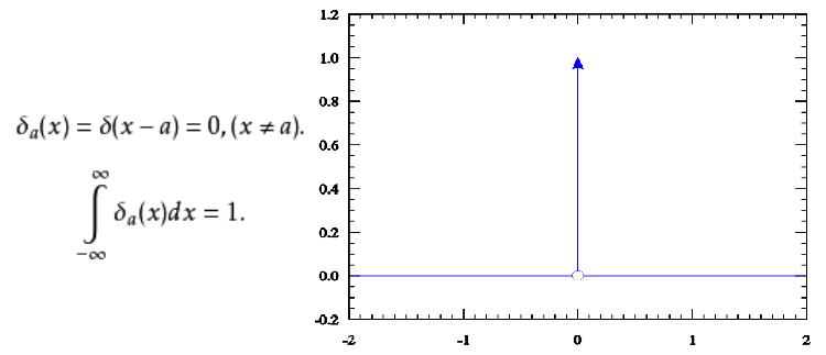
当 $\mathcal{A}=\mathbb{R}^{n}$: 时任意连续可微, 总积分为 1 ，并且紧支撑的 $\xi$ : $\mathbb{R}^{n}\rightarrow \mathbb{R}$, 能够构建出 $\nu_{\sigma}(a’,\ a)=1/\sigma^{n}\xi((a-a’)/\sigma)$，这满足条件B1。并且这样的函数范围很大：给出任意紧支撑这个函数都能构建出来。

条件1，$\int_\mathcal{A}\nu_\delta(a’,\ a) da=\int_\mathcal{A}1/\sigma^{n}\xi((a-a’)/\sigma)da=\int_\mathcal{A}\xi((a-a’)/\sigma)d((a-a’)/\sigma)=1$，当$a-a’\neq 0$，存在$\sigma>0$使得$(a-a’)/\sigma=0$，即$\lim_{\sigma\downarrow 0}(1/\sigma^{n}\xi((a-a’)/\sigma))=0$。$\lim_{\sigma\downarrow 0}\nu(a’,x)=\delta_a’(x)$。条件2,3,4显然成立。

引理1。

当 $\mathcal{U}\times \mathcal{V}\subseteq \mathbb{R}^{n}\times \mathbb{R}^{n}$，并且 $\nu$ : $\mathcal{U}\times \mathcal{V}\rightarrow \mathbb{R}$ 在 $\mathcal{U}\times \mathcal{V}$上可微分。故有 $(A)\Leftrightarrow(B)\Rightarrow(C)$，

(A) 对所有 $u\in \mathcal{U}, v\in \mathcal{V}$, $\delta\in \mathbb{R}^{n}$ 有 $u+\delta\in \mathcal{U}, v+\delta\in \mathcal{V}, \nu(u,\ v)=\nu(u+\delta,\ v+\delta)$。
(B) 存在函数 $\chi$ : $\mathbb{R}^{n}\rightarrow \mathbb{R}$ 有 $\nu(u,\ v)=\chi(u-v)$。
(C) $\nabla_{u}\nu(u,\ v)=-\nabla_{v}\nu(u,\ v)$，梯度处处存在。
另外，如果 $\mathcal{U}\times \mathcal{V}$ 是凸集，则有 $C\Rightarrow \mathrm{A}$。
引理${\it proof}$。
$\mathrm{A}\Rightarrow \mathrm{B}$:

$$\begin{split} \chi(u-v)&=\nu(u,\ u-(u-v))\\ &=\nu(u,\ v) \end{split}$$

$\mathrm{B}\Rightarrow \mathrm{A}$:

$$\begin{split} \nu(u,\ v)&=\chi(u-v)\\ &=\chi((u+\delta)-(v+\delta))\\ &=\nu(u+\delta,\ v+\delta) \end{split}$$

$\mathrm{B}\Rightarrow \mathrm{C}$: 令 $h(u,\ v)=u-v$ 根据链式法则，

$$\nabla_{u}u(u,\ v)\!=\!\nabla_{h}\chi(h)|_{h(u,v)}\!\nabla_{u}h(u,\ v)\!=\!\nabla_{h}\chi(h)|_{h(u,v)}\!=\! -\!\nabla_{h}\chi(h)|_{h(u,v)}\!\nabla_{v}h(u,\ v)\!=\!-\nabla_{v}\nu(u,\ v)$$

($\mathrm{C}$ 和凸集) $\Rightarrow \mathrm{A}$: 假设 $\mathcal{U}\times \mathcal{V}$ 是凸集。对任何 $(u,\ v)\in \mathcal{U}\times \mathcal{V}$, $\delta\in \mathbb{R}^{n}$, 有，

$$\begin{split} \langle\nabla_{(u,v)}\nu(u,\ v)\ ,\ (\delta,\ \delta)\rangle&=\langle\nabla_{u}\nu(u,\ v)\ ,\ \delta\rangle+\langle\nabla_{v}\nu(u,\ v)\ ,\ \delta\rangle\\ &=\langle\nabla_{u}\nu(u,\ v)\ ,\ \delta\rangle-\langle\nabla_{u}\nu(u,\ v)\ ,\ \delta\rangle\\ &=0 \end{split}$$

因为 $\mathcal{U}\times \mathcal{V}$ 是凸集, 对任意 $A=(u,\ v)\in \mathcal{U}\times \mathcal{V}$ 和 $B=(u+\delta,\ v+\delta)\in \mathcal{U}\times \mathcal{V}$ 有直线连接 $A$ 和 $B$ ，这条直线式是完全包含在 $\mathcal{U}\times \mathcal{V}$中的。 因此 $\nu$ 沿着这条线就有 $\nu(A)=\nu(B)$。

引理2。

1. 对于任意 $\pi,\ t,\ \displaystyle \sup_{s}p_{t}^{\pi}(s)<b$。
2. 对于任意 $\pi, \displaystyle \sup_{s}\rho^{\pi}(s)<b/(1-\gamma)$。
3. 对于任意 $\pi, \displaystyle \sup_{a,s}||\nabla_{a}Q^{\pi}(a,\ s)||<c<\infty$。
$\it Proof$. 1. 当 $t=1$ 常规条件 A.2, 当 $t\geq 1,$

$$\sup_{s'}p_{t+1}^{\pi}(s')=\sup_{s'}\int p_{t}^{\pi}(s)\int\pi_\theta(a,\ s)p(s'|s,\ a)dads=\sup_{s'}\mathrm{E}_{s\sim p_{t}^{\pi},a\sim\pi_{\theta}}\left[p(s'|s,\ a)\right]$$ $$\leq\sup_{s,a,s}p(s'|s,\ a)<b$$

2. $\displaystyle \sup_{s}\rho^{\pi}(s)\leq\sum_{t=1}^{\infty}\gamma^{t-1}\sup_{s}p_{t}^{\pi}(s)\leq b/(1-\gamma)$
$\displaystyle \sup_{s}V^{\pi}(s)\leq\sum_{t=1}^{\infty}\gamma^{t-1}\sup_{s}r(s_{k},\ a_{k})\leq b/(1-\gamma)$

3. 有,

$$\sup_{s,a}\left \|\nabla_{a}Q^{\pi}(a,\ s)\right \|\leq\sup_{s,a}\left \|\nabla_{a}r(s,\ a)\right \|+\gamma\sup_{s,a}\int\left \|\nabla_{a}p(s'|s,\ a)\right \|\left|V^{\pi}(s')\right|ds'$$ $$\leq L+\gamma\int Lb/(1-\gamma)ds'$$ $$<\infty$$

因为 $S$ 紧的，并且在 $S$ 上的积分时有限的。

引理3。

$\displaystyle \lim_{\sigma\downarrow 0}\rho^{\pi_{\mu_{\theta},\sigma}}(s)=\rho^{\pi_{\mu_{\theta},0}}(s)$ 并且收敛是一致收敛,

$$\displaystyle \lim_{\sigma\downarrow 0}\sup_{s}|\rho^{\pi_{\mu_{\theta},\sigma}}(s)-\rho^{\pi_{\mu_{\theta},0}}(s)|=0$$

$\it Proof.$ 我们有 $\displaystyle \rho^{\pi}(s)=\sum_{t=1}^{\infty}\gamma^{t-1}p_{t}^{\pi}(s)$。显然有 $p_{1}^{\pi_{\mu_{\theta},\sigma}}(s)=p_{1}(s)=p_{1}^{\pi_{\mu_{\theta},0}}(s)$。对应 $\nu_{\sigma}$ 的定义，对应任意 $\epsilon_{1}>0$ 存在 $\sigma^{*}$ 当 $\sigma<\sigma^{*}$时，

$$\sup_{s}\left|\int\pi_{\mu_{\theta},\sigma}(a|s)p(s'|s,\ a)da-\int\pi_{\mu_{\theta},0}(a|s)p(s'|s,\ a)da\right|\leq\epsilon_{1}.$$

现在假设 $t\geq 1$ 时有

$$\sup_{s}\left|p_{t}^{\pi_{\mu_{\theta},\sigma}}(s)-p_{t}^{\pi_{\mu_{\theta},0}}(s)\right|\leq\epsilon_{2}(t)\ ,$$

则,

$$\begin{split} &\sup_{s'}\left|p_{t+1}^{\pi_{\mu_{\theta},\sigma}}(s')-p_{t+1}^{\pi_{\mu_{\theta},0}}(s')\right|\\ &\leq\sup_{s'}\left|\int\int p_{t}^{\pi_{\mu_{\theta},\sigma}}(s)\pi_{\mu_{\theta},\sigma}(a|s)p(s'|s,\ a)dads-\int\int p_{t}^{\pi_{\mu_{\theta},0}}(s)\pi_{\mu_{\theta},0}(a|s)p(s'|s,\ a)dads\right|\\ &\leq\sup_{s'}\int\left|p_{t}^{\pi_{\mu_{\theta},\sigma}}(s)-p_{t}^{\pi_{\mu_{\theta},0}}(s)\right|\int\pi_{\mu_{\theta},\sigma}(a|s)p(s'|s,\ a)dads\\ &+\sup_{s'}\int p_{t}^{\pi_{\mu_{\theta},0}}(s)\left|\int\pi_{\mu_{\theta},\sigma}(a|s)p(s'|s,\ a)da-\int\pi_{\mu_{\theta},0}(a|s)p(s'|s,\ a)da\right|ds\\ &\leq\epsilon_{2}(t)\int bds+\epsilon_{1}\\ &=\epsilon_{2}(t)b\zeta+\epsilon_{1}, \end{split}$$

这里 $\displaystyle \zeta=\int 1ds<\infty$. 因为 $\epsilon_{2}(1)=0$ 有，

$$\sup_{s}\left|p_{1}^{\pi_{\mu_{\theta},\sigma}}(s)-p_{1}^{\pi_{\mu_{\theta},0}}(s)\right|\leq 0\leq\epsilon_{1}$$

假设，

$$\sup_{s}\left|p_{t}^{\pi_{\mu_{\theta},\sigma}}(s)-p_{t}^{\pi_{\mu_{\theta},0}}(s)\right|\leq\epsilon_{1}(b\zeta+1)^{t-1}$$

t+1时，

$$\begin{split} \sup_{s}\left|p_{t+1}^{\pi_{\mu_{\theta},\sigma}}(s)-p_{t+1}^{\pi_{\mu_{\theta},0}}(s)\right|&\leq\epsilon_{1}(b\zeta+1)^{t-1}b\zeta+\epsilon_{1}\\ &\leq\epsilon_{1}((b\zeta+1)^{t-1}b\zeta+1)\\ &\leq\epsilon_{1}((b\zeta+1)^{t-1}b\zeta+(b\zeta+1)^{t-1})\\ &\leq\epsilon_{1}(b\zeta+1)^{(t+1)-1} \end{split}$$

故有

$$\sup_{s}\left|p_{t}^{\pi_{\mu_{\theta},\sigma}}(s)-p_{t}^{\pi_{\mu_{\theta},0}}(s)\right|\leq\epsilon_{1}(b\zeta+1)^{t-1}$$

对于任意 $\epsilon>0$ 可以选择一个足够大的 $T$ 使得 $\displaystyle \sum_{t=T+1}^{\infty}\gamma^{t-1}b<\epsilon/2$ 然后选择 $\sigma^{*}$ 使得 $\epsilon_{1}$ 足够小使得 $\displaystyle \sum_{t=1}^{T}\gamma^{t-1}\epsilon_{1}(b\zeta+1)^{t-1}<\epsilon/2$, 这样对应任意 $\sigma<\sigma^{*}$ 有，

$$\begin{split} \sup_{s}\left|\rho^{\pi_{\mu_{\theta},\sigma}}(s)-\rho^{\pi_{\mu_{\theta},0}}(s)\right|&=\sup_{s}\left|\sum_{t=1}^{\infty}\gamma^{t-1}p_{t}^{\pi_{\mu_{\theta},\sigma}}(s)-\sum_{t=1}^{\infty}\gamma^{t-1}p_{t}^{\pi_{\mu_{\theta},0}}(s)\right|\\ &\leq\sum_{t=1}^{T}\gamma^{t-1}\sup_{s}\left|p_{t}^{\pi_{\mu_{\theta},\sigma}}(s)-p_{t}^{\pi_{\mu_{\theta},0}}(s)\right|\\ &+\sum_{t=T+1}^{\infty}\gamma^{t-1}\sup_{s}\left|p_{t}^{\pi_{\mu_{\theta},\sigma}}(s)-p_{t}^{\pi_{\mu_{\theta},0}}(s)\right|\\ &\leq\sum_{t=1}^{T}\gamma^{t-1}\epsilon_{1}(b\zeta+1)^{t-1}+\sum_{t=1}^{\infty}\gamma^{t-1}b\\ &\leq\epsilon \end{split}$$

引理 4.

对于所有 $s\in S,\ \theta$，当 $\sigma\rightarrow 0$ 时 $\nabla_{a}Q^{\pi_{\mu_{\theta},\sigma}}(a,\ s)\rightarrow\nabla_{a}Q^{\pi_{\mu_{\theta},0}}(a,\ s)$，并且在 $(s,\ a)$ 上一致收敛。

$$\lim_{\sigma\downarrow 0}\sup_{(s,a)}\left\|\nabla_{a}Q^{\pi_{\mu_{\theta},\sigma}}(a,\ s)-\nabla_{a}Q^{\pi_{\mu_{\theta},0}}(a,\ s)\right\|=0$$

$Proof.$ $\displaystyle \nabla_{a}Q^{\pi}(a,\ s)=\nabla_{a}(r(s,\ a)+\gamma\int p(s’|s,\ a)V^{\pi}(s’)ds’)$ ，所以有，

$$\begin{split} \sup_{(s,a)}\left\|\nabla_{a}Q^{\pi_{\mu_{\theta},\sigma}}(a,\ s)-\nabla_{a}Q^{\pi_{\mu_{\theta},0}}(a,\ s)\right\|&\leq\gamma\int\sup_{(s,s',a)}\left\|\nabla_{a}p(s'|s,\ a)\right\|\left|V^{\pi_{\mu_{\theta},\sigma}}(s')-V^{\pi_{\mu_{\theta},0}}(s')\right|ds'\\ &\leq\gamma\zeta L\sup_{s'}\left|V^{\pi_{\mu_{\theta},\sigma}}(s')-V^{\pi_{\mu_{\theta},0}}(s')\right| \end{split}$$

这里 $\displaystyle \zeta=\int 1ds<\infty$. 对任意 $\epsilon_{1}, \epsilon_{2}$ 存在 $\sigma^{*}$ 对所有 $\sigma<\sigma^{*}$ 都有，

$$\sup_{s}\left|\int r(s,\ a)(\pi_{\mu_{\theta},\sigma}(a|s)-\pi_{\mu_{\theta},0}(a|s))da\right|<\epsilon_{1}$$

和

$$\displaystyle \sup_{s,\hat{s}}\left|\rho_{\hat{s}}^{\pi_{\mu_{\theta},\sigma}}(s)-\rho_{\hat{s}}^{\pi_{\mu_{\theta},0}}(s)\right|<\epsilon_{2}$$

这里 $\rho_{\hat{s}}^{\pi}(s)$ 和 $\rho^{\pi}(s)$，相似，只是在 $t=1$ 时的分布是 $\displaystyle \int p(s|a,\hat{s})\pi(a|\hat{s})da$ 而不是 $p_{1}$。然后有，

$$\begin{split} &\sup_{s'}\left|V^{\pi_{\mu_{\theta},\sigma}}(s')-V^{\pi_{\mu_{\theta},0}}(s')\right|\\ &\leq\sup_{s'}\left|\int r(s',\ a)(\pi_{\mu_{\theta},\sigma}(a|s')-\pi_{\mu_{\theta},0}(a|s'))da\right|\\ &+\displaystyle \gamma\sup_{s'}\left|\int\int\rho_{s'}^{\pi_{\mu_{\theta},\sigma}}(s)\pi_{\mu_{\theta},\sigma}(a|s)r(s,\ a)dads-\int\int\rho_{s'}^{\pi_{\mu_{\theta},0}}(s)\pi_{\mu_{\theta},0}(a|s)r(s,\ a)dads\right|\\ &\leq\epsilon_{1}+\sup_{s'}\int\int\left|\rho_{s'}^{\pi_{\mu_{\theta},\sigma}}(s)-\rho_{s'}^{\pi_{\mu_{\theta},0}}(s)\right|\left|r(s,\ a)\right|\pi_{\mu_{\theta},\sigma}(a|s)dads\\ &+\left|\sup_{s'}\int\rho_{s'}^{\pi_{\mu_{\theta},0}}(s)\int r(s,\ a)(\pi_{\mu_{\theta},\sigma}(a|s)-\pi_{\mu_{\theta},0}(a|s))dads\right|\\ &\leq\epsilon_{1}+\epsilon_{2}\zeta b+\epsilon_{1}/(1-\gamma) \end{split}$$

其中，$\displaystyle \sup_{s}\int\rho^{\pi}(s)ds\leq\sum_{t=1}^{\infty}\gamma^{t-1}\sup_{s}\int p_{t}^{\pi}(s)ds\leq 1/(1-\gamma)$ 。最后要通过选择 $\sigma$ 就可以任意小。

证明极限要用到的定理总结：

B1条件：

$$\lim_{\sigma\downarrow 0}\int_{A}\nu_{\sigma}(a',\ a)f(a)da=f(a')$$

引理1:

$$\nabla_{u}\nu(u,\ v)=-\nabla_{v}\nu(u,\ v)$$

引理3：

$$\lim_{\sigma\downarrow 0}\rho^{\pi_{\mu_{\theta},\sigma}}(s)=\rho^{\pi_{\mu_{\theta},0}}(s)$$

引理4：

$$\lim_{\sigma\downarrow 0}\sup_{(s,a)}\left\|\nabla_{a}Q^{\pi_{\mu_{\theta},\sigma}}(a,\ s)-\nabla_{a}Q^{\pi_{\mu_{\theta},0}}(a,\ s)\right\|=0$$

$\it proof$ 理论。

由于引理1中 $\nabla_{a’}\nu_{\sigma}(a’,\ a)|_{a’=\mu_{\theta}(s)}=-\nabla_{a}\nu_{\sigma}(\mu_{\theta}(s),\ a)$ . 所以有,

$$\begin{split} &\int_{A}Q^{\pi_{\mu_{\theta,\sigma}}}(s,\ a)\nabla_{a'}\nu_{\sigma}(a',\ a)|_{a'=\mu_{\theta}(s)}da\\ &=-\displaystyle \int_{A}Q^{\pi_{\mu_{\theta,\sigma}}}(s,\ a)\nabla_{a}\nu_{\sigma}(\mu_{\theta}(s),\ a)\mathrm{d}a\\ &=\displaystyle \int_{C_{\mu_{\theta}(\mathrm{s})}}\nabla_{a}Q^{\pi_{\mu_{\theta},\sigma}}(s,\ a)\nu_{\sigma}(\mu_{\theta}(s),\ a)\mathrm{d}a+ boundary\ terms\\ &=\int_{C_{\mu_{\theta}(\mathrm{s})}}\nabla_{a}Q^{\pi_{\mu_{\theta},\sigma}}(s,\ a)\nu_{\sigma}(\mu_{\theta}(s),\ a)\mathrm{d}a \end{split}$$

因为 $\nu_{\sigma}$ 在边界上消失了所以boundary terms为零。对于随机策略有，

$$\begin{split} \displaystyle \lim_{\sigma\downarrow 0}\nabla_{\theta}J(\pi_{\mu_{\theta},\sigma})&=\lim_{\sigma\downarrow 0}\int_{\mathcal{S}}\rho^{\pi_{\mu_{\theta},\sigma}}(s)\int_{A}Q^{\pi_{\mu_{\theta},\sigma}}(s,\ a)\nabla_{\theta}\pi_{\mu_{\theta},\sigma}(a|s)dads\\ &=\displaystyle \lim_{\sigma\downarrow 0}\int_{\mathcal{S}}\rho^{\pi_{\mu_{\theta},\sigma}}(s)\int_{A}Q^{\pi_{\mu_{\theta},\sigma}}(s,\ a)\nabla_{\theta}\mu_{\theta}(s)\nabla_{a'}\nu_{\sigma}(a',\ a)|_{a=\mu_{\theta}(s)}dads\\ &=\displaystyle \lim_{\sigma\downarrow 0}\int_{\mathcal{S}}\rho^{\pi_{\mu_{\theta},\sigma}}(s)\nabla_{\theta}\mu_{\theta}(s)\int_{C_{\mu_{\theta}(s)}}\nabla_{a}Q^{\pi_{\mu_{\theta},\sigma}}(s,\ a)\nu_{\sigma}(\mu_{\theta}(s),\ a)dads\\ &=\displaystyle \int_{\mathcal{S}}\lim_{\sigma\downarrow 0}\rho^{\pi_{\mu_{\theta},\sigma}}(s)\nabla_{\theta}\mu_{\theta}(s)\int_{C_{\mu_{\theta}(s)}}\nabla_{a}Q^{\pi_{\mu_{\theta},\sigma}}(s,\ a)\nu_{\sigma}(\mu_{\theta}(s),\ a)dads \end{split}\tag{6}$$

在 (6) 按照显著收敛理论交换了积分和极线。根据引理显著函数为,

$$\begin{split} g_{\theta}(s)&=\sup_{\sigma}\{\rho^{\pi_{\mu_{\theta},\sigma}}(s)\}\sup_{a\in C_{\mu_{\theta}(s)},\sigma}\{\left\|\nabla_{a}Q^{\pi_{\mu_{\theta},\sigma}}(a,\ s)\right\|\}\left\|\nabla_{\theta}\mu_{\theta}(s)\right\|_{\mathrm{o}\mathrm{p}}\\ &\displaystyle \geq\left\|\rho^{\pi_{\mu_{\theta},\sigma}}(s)\int_{C_{\mu_{\theta}(s)}}\nabla_{a}Q^{\pi_{\mu_{\theta},\sigma}}(s,\ a)\nu_{\sigma}(\mu_{\theta}(s),\ a)\mathrm{d}a\nabla_{\theta}\mu_{\theta}(s)\right\| \end{split}\tag{7}$$

这里 $||\cdot||_{\mathrm{o}\mathrm{p}}$ 表示 operator norm, 或是最大的奇异值。
operator norm的定义: $\left|A\right|_{op}=\inf\{c\geq 0:\left|A\nu\right|\leq c\left|\nu\right|\ for\ all\ \nu\in\mathcal{V}\}$
引理4中证明了 $\nabla_{a}Q^{\pi_{\mu_{\theta},\sigma}}(s,\ a)$ 的一致收敛，对应任意 $\epsilon_{1}, \epsilon_{2}$ 存在 $\sigma^{*}$ 对应任意 $\sigma<\sigma^{*}$ 有，

$$\left\|\nabla_{a}Q^{\pi_{\mu_{\theta},\sigma}}(s,\ a)-\nabla_{a}Q^{\pi_{\mu_{\theta},0}}(s,\ a)\right\|<\epsilon_{1}$$

所以有，

$$\left\|\int_{C_{\mu_{\theta}(s)}}\nabla_{a}Q^{\pi_{\mu_{\theta},\sigma}}(s,\ a)\nu_{\sigma}(\mu_{\theta}(s),\ a)\mathrm{d}a-\int_{C_{\mu_{\theta}(s)}}\nabla_{a}Q^{\pi_{\mu_{\theta},0}}(s,\ a)\nu_{\sigma}(\mu_{\theta}(s),\ a)\mathrm{d}a\right\|<\epsilon_{1},$$

又因为有(B1),

$$\left\|\int_{C_{\mu_{\theta}(s)}}\nabla_{a}Q^{\pi_{\mu_{\theta},0}}(s,\ a)\nu_{\sigma}(\mu_{\theta}(s),\ a)\mathrm{d}a-\nabla_{a}Q^{\pi_{\mu_{\theta},0}}(s,\ a)|_{a=\mu_{\theta}(s)}\right\|<\epsilon_{2}.$$

因此,

$$\left\|\int_{C_{\mu_{\theta}(s)}}\nabla_{a}Q^{\pi_{\mu_{\theta},\sigma}}(s,\ a)\nu_{\sigma}(\mu_{\theta}(s),\ a)\mathrm{d}a-\nabla_{a}Q^{\pi_{\mu_{\theta},0}}(s,\ a)|_{a=\mu_{\theta}(s)}\right\|<\epsilon_{1}+\epsilon_{2}$$

从这里和引理3可以得到,

$$\begin{split} (6)&=\displaystyle \int_{\mathcal{S}}\rho^{\pi_{\mu_{\theta},0}}(s)\nabla_{\theta}\mu_{\theta}(s)\lim_{\sigma\downarrow 0}\int_{C_{\mu_{\theta}(s)}}\nabla_{a}Q^{\pi_{\mu_{\theta},\sigma}}(s,\ a)\nu_{\sigma}(\mu_{\theta}(s),\ a)d{\it a}ds\\ &=\int_{\mathcal{S}}\rho^{\pi_{\mu_{\theta},0}}(s)\nabla_{\theta}\mu_{\theta}(s)\nabla_{a}Q^{\pi_{\mu_{\theta},0}}(s,\ a)|_{a=\mu_{\theta}(s)}\mathrm{d}s\\ &=\int_{\mathcal{S}}\rho^{\mu_{\theta}}(s)\nabla_{\theta}\mu_{\theta}(s)\nabla_{a}Q^{\mu_{\theta}}(s,\ a)|_{a=\mu_{\theta}(s)}\mathrm{d}s \end{split}$$

5. Compatible Function Approximation

近似函数 $Q^{w}(s,\ a)$ 可兼容的条件，

1. $\nabla_{a}Q^{w}(s,\ a)|_{a=\mu_{\theta}(s)}=\nabla_{\theta}\mu_{\theta}(s)^{\mathrm{T}}w$
2. $w$ 最小化了平方差 $MSE(\theta,\ w)= \mathrm{E}[\epsilon(s;\theta,\ w)^{\mathrm{T}}\epsilon(s;\theta,\ w)]$ 其中 $\epsilon(s;\theta,\ w) =\nabla_{a}Q^{w}(s,\ a)|_{a=\mu_{\theta}(s)}-\nabla_{a}Q^{\mu}(s,\ a)|_{a=\mu_{\theta}(s)}$

$\it Proof$. 如果 $w$ 最小化了 $MSE$，这时 $\epsilon^{2}$ 相对于 $w$ 的梯度必须为零。又因为条件1有 $\nabla_{w}\epsilon(s;\theta,\ w)=\nabla_{\theta}\mu_{\theta}(s)$ ,

$$\begin{split} \nabla_{w}MSE(\theta,\ w)&=0\\ \mathrm{E}[\nabla_{\theta}\mu_{\theta}(s)\epsilon(s;\theta,\ w)]&=0\\ \mathrm{E}[\nabla_{\theta}\mu_{\theta}(s)\nabla_{a}Q^{w}(s,\ a)|_{a=\mu_{\theta}(s)}]&=\\ \mathrm{E}[\nabla_{\theta}\mu_{\theta}(s)\nabla_{a}Q^{\mu}(s,\ a)|_{a=\mu_{\theta}(s)}]&=\nabla_{\theta}J_{\beta}(\mu_{\theta})\ or\ \nabla_{\theta}J(\mu_{\theta})\end{split}$$

这时取 $Q^{w}(s,\ a)= (a-\mu_{\theta}(s))^{\mathrm{T}}\nabla_{\theta}\mu_{\theta}(s)^{\mathrm{T}}w+V^{v}(s)$ 能满足条件1。在使用Sarsa或Q-learning时有 $Q^{w}(s,\ a)\approx Q^{\mu}(s,\ a)$，因为平滑函数近似 $\nabla_{a}Q^{w}(s,\ a)|_{a=\mu_{\theta}(s)}\approx \nabla_{a}Q^{\mu}(s,\ a)|_{a=\mu_{\theta}(s)}$。这样满足了条件2。

6. DDPG

改进

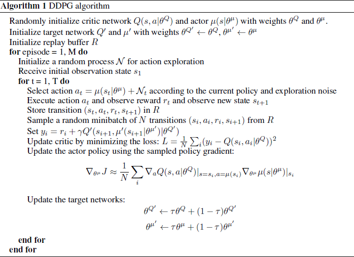
1. 样本缓存池
2. 加目标网络，延迟更新：
$\theta^{Q’}\leftarrow\tau\theta^{Q}+(1-\tau)\theta^{Q’},\\
\theta^{\mu’}\leftarrow\tau\theta^{\mu}+(1-\tau)\theta^{\mu’}$
3. 加入探索噪声：
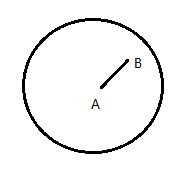
Ornstein-Uhlenbeck process，$dx_t=\theta(\mu-x_t)dt+\sigma dW_t$。这是一个随机微分函数。

其中$\theta=1.0,\ \sigma=300,\ \mu=(0,\ 0)$初始位置在$(10,\ 10)$。

4. 状态变量尺度不同：batch normalization
5. 用像素做输入。

伪代码

实验

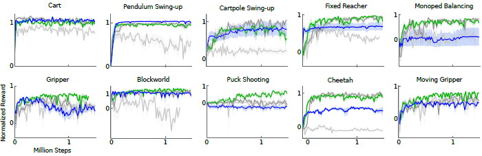
亮灰色：使用batch normalization的原始DPG。
暗灰色：有目标网络。
绿色：有目标网络和batch normalization。
蓝色：像素输入和目标网络。

Reference:
Deterministic Policy Gradient Algorithms.
Continuous control with deep reinforcement learning.